Diffusion MRI Fundamentals

This page summarises the imaging physics csttool depends on. It is adapted from the corresponding chapter of the thesis (Nalo, 2026) and follows the same notation. For a deeper treatment, see Soares et al., 2013.

Diffusion and tissue microstructure

Diffusion-weighted imaging (DWI) generates image contrast from the diffusion of water molecules. Diffusion — Brownian motion — refers to the random thermal movement of particles. In a homogeneous medium, diffusion is isotropic: equal in all directions. In biological tissue, cellular structures such as membranes, organelles and (in white matter) axonal walls and myelin sheaths hinder free motion, so diffusion becomes anisotropic. The degree and orientation of this anisotropy reflect tissue microstructure and change under pathological conditions, which makes DWI an essential tool in neuroimaging.

How diffusion contrast is generated

To sensitise the MR signal to diffusion, a pair of diffusion gradients (DGs) is applied around a refocusing 180° pulse in a spin-echo sequence. For stationary spins, the phase accumulated under the first gradient is fully reversed by the second. For diffusing spins, however, the spin has moved to a different magnetic environment in the interval between the two gradients, so refocusing is incomplete and the signal decays. This creates contrast between stationary and diffusing populations.

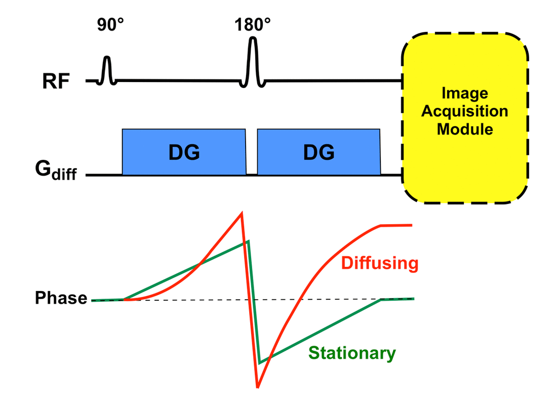
Effect of diffusion gradients on stationary and diffusing spins. Figure courtesy of Allen D. Elster, MRIquestions.com.

The b-value

The strength of the diffusion weighting is controlled by the operator through the b-value, which governs how quickly the signal decays:

$$ S(b) = S_0 \exp(-bD) $$

where $S_0$ is the signal without diffusion weighting and $D$ is the diffusion coefficient. For rectangular pulses (Stejskal & Tanner, 1965):

$$ b = \gamma^2 G^2 \delta^2 (\Delta - \delta/3) $$

with $\gamma$ the gyromagnetic ratio, $G$ the gradient amplitude, $\delta$ the gradient duration, and $\Delta$ the inter-gradient interval. The b-value has units of s/mm². Routine clinical DWI uses b-values in the 0–1000 s/mm² range, with 1000 s/mm² being the standard for many pathologies (Kazemzadeh et al., 2025).

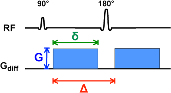
Illustration of the b-value parameters. Figure courtesy of Allen D. Elster, MRIquestions.com.

The diffusion tensor

The scalar diffusion coefficient $D$ is an over-simplification: it assumes isotropic motion. The diffusion tensor $\mathcal{D}$ extends $D$ by encoding both magnitude and direction:

$$ \mathcal{D} = \begin{bmatrix} D_{xx} & D_{xy} & D_{xz} \ D_{yx} & D_{yy} & D_{yz} \ D_{zx} & D_{zy} & D_{zz} \end{bmatrix} $$

Eigenvalue decomposition yields three eigenvectors $\mathbf{v}_i$ (principal directions of diffusion) and eigenvalues $\lambda_i$ (their magnitudes). Geometrically, this maps to an ellipsoid oriented along $\mathbf{v}_i$ and scaled by $\sqrt{\lambda_i}$.

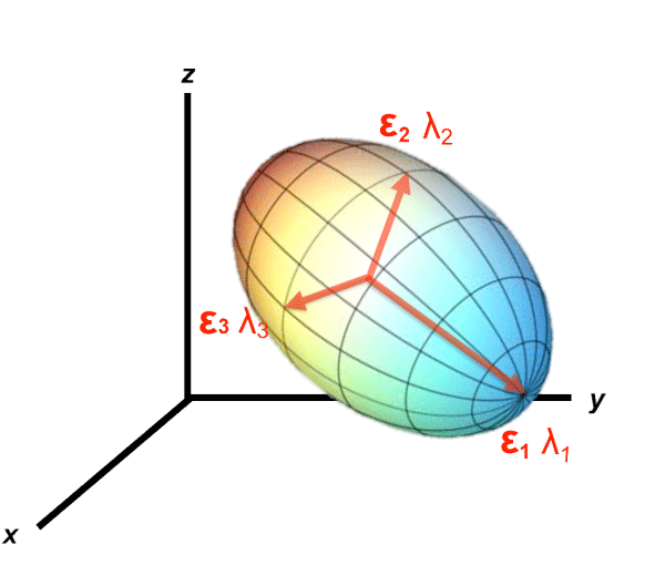
Diffusion ellipsoid with eigenvector directions $\mathbf{\epsilon}_i$ and eigenvalue magnitudes $\lambda_i$. Figure courtesy of Allen D. Elster, MRIquestions.com.

A minimum of six gradient directions are required to fit the tensor; in practice ≥30 (preferably ≥64) are used to suppress error from crossing, kissing or branching fibres.

DTI scalar metrics

Diffusion tensor imaging (DTI) summarises the tensor with four scalars. csttool reports all four.

Metric	Definition	Interpretation
Axial diffusivity (AD)	$\lambda_1$	Diffusion along the principal axis.
Radial diffusivity (RD)	$(\lambda_2 + \lambda_3)/2$	Mean perpendicular diffusion.
Mean diffusivity (MD)	$(\lambda_1 + \lambda_2 + \lambda_3)/3$	Direction-independent average.
Fractional anisotropy (FA)	$\sqrt{\frac{(\lambda_1-\lambda_2)^2 + (\lambda_2-\lambda_3)^2 + (\lambda_3-\lambda_1)^2}{2(\lambda_1^2 + \lambda_2^2 + \lambda_3^2)}}$	Relative anisotropy in $[0, 1]$.

In healthy adult white matter, typical CST values at 3 T are FA ≈ 0.58, MD ≈ 0.79 × 10⁻³ mm²/s, AD ≈ 1.4 × 10⁻³ mm²/s, RD ≈ 0.50 × 10⁻³ mm²/s (Reich et al., 2006). In ALS, FA decreases and MD/RD increase along the CST relative to controls, reflecting loss of axonal integrity (Sarica et al., 2017).

DTI limitations in crossing-fibre voxels

FA is a relative measure and can behave counter-intuitively in voxels containing crossing fibres (Figley et al., 2022).

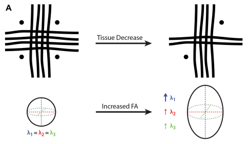
Left: FA = 0 (no dominant direction). Right: fibre loss causes $\lambda_1$ to increase relative to $\lambda_2$ and $\lambda_3$, raising FA despite a net loss of tissue.

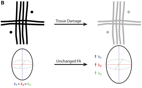
Left: a principal orientation gives FA > 0. Right: proportional degradation of all eigenvalues leaves FA unchanged despite microstructural damage. Figures adapted from Figley et al., 2022.

These limitations do not disqualify DTI: non-relative metrics such as MD or the trace ($\lambda_1 + \lambda_2 + \lambda_3$) are more robust in crossing-fibre regions, and the CST itself is anatomically simple enough that crossing-fibre confounds are limited. Clinical interpretation should always corroborate DTI with other imaging metrics.

Software used

• DIPY (Garyfallidis et al., 2014) — tensor fitting, scalar metrics.
• Patch2Self denoising — see the preprocess reference.

See Tractography for how the principal eigenvectors are turned into 3D streamlines, and CST Anatomy for the anatomical context.